Light Propagation Volumes

Light Propagation Volumes (LPV) is an algorithm for achieving an indirect light bounce developed by Crytek and (previously) used in CryEngine 3. Having read numerous papers and articles (listed below), looked through code on GitHub (also listed below), I was disapppointed that there was a lack of clear information on how the algorithm works technically. This article aims to provide an insight in how the algorithm works and how I have implemented it in the engine I am working on for a school project.

What does LPV do?

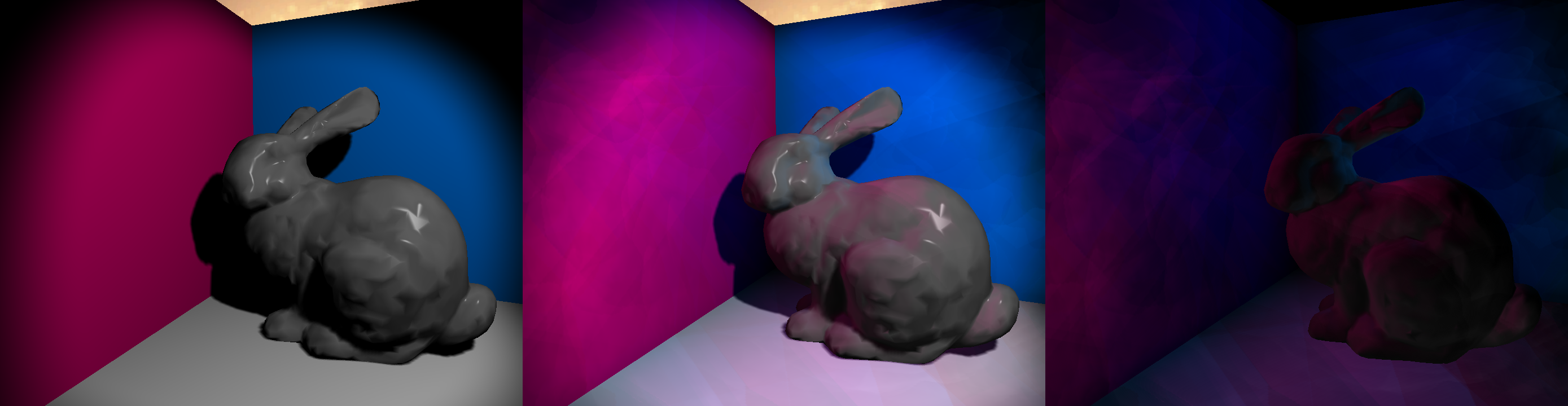
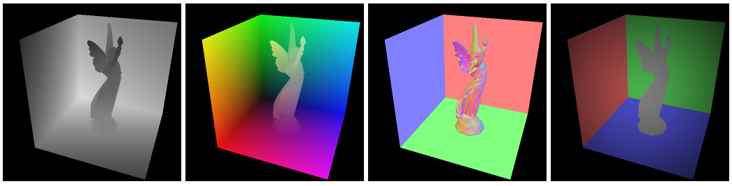
Light Propagation Volumes stores lighting information from a light in a 3D grid. Every light stores which points in the world they light up. These points have a coordinate in the world, which means you can stratify those coordinates in a grid. In that way you save lit points (Virtual Point Lights) in a 3D grid and can use those initial points to spread light across the scene. You can imagine the spreading of lights as covering your sandwich in Nutella. You start off with an initial lump of Nutella (virtual point lights) and use a knife to spread (propagate) this across the entire sandwich (the entire scene). It’s a bit more complex than that, but that will become clear very soon. The images below demonstrates what LPV adds to a scene.

lpv_comparison

How does it do that?

Injection

The first step is to gather the Virtual Point Lights (VPLs). In a previous article I describe Reflective Shadow Maps. For my implementation I used the flux, world-space position, and world-space normal map resulting from rendering the Reflective Shadow Map. The flux is the color of the indirect light getting injected, the world-space position is used to determine the grid cell, and the normal determines the initial propagation direction.

Not every pixel in the RSM will be used for injection in the grid, because this would mean you inject 2048×2048=4194304 VPLs for a decently sized RSM for a directional light. Performance was decent, but that was only with one light. Some intelligent down-sampling (to 512×512) still gives pretty and stable results.

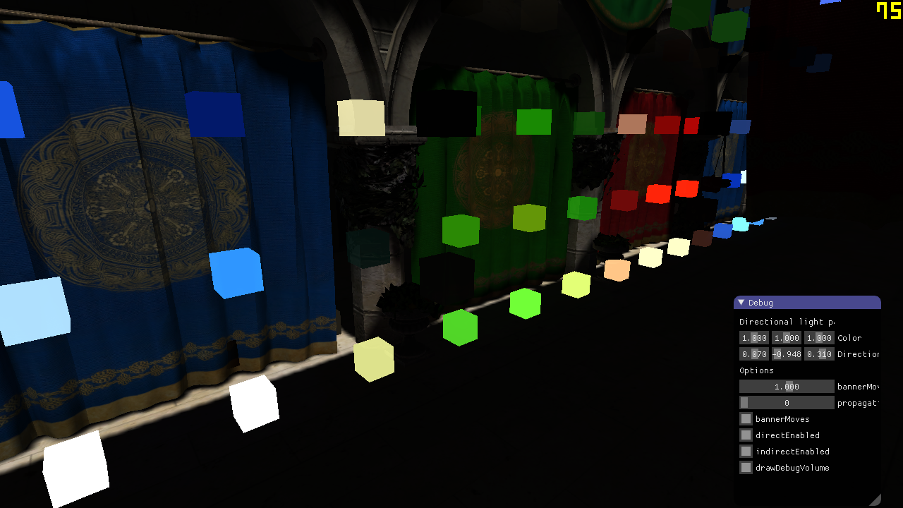
The image below demonstrates the resulting 3D grid after the Injection phase. With a white light, the colors of the VPLs are very similar to the surface they are bounced off of.

Demo_2016-06-27_20-29-44

Storage

To maximize efficiency and frame rate, the algorithm stores the lighting information in Spherical Harmonics (SH). Those are mathematical objects used to record an incoming signal (like light intensity) over a sphere. The internal workings of this are still a bit of a mystery to me, but important is to know that you can encode light intensities and directions in Spherical Harmonics, allowing for propagation using just 4 floats per color channel. Implementation details will become apparent soon.

Propagation

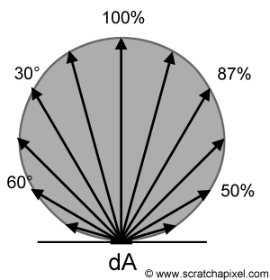
So, we have a grid filled with Virtual Point Lights and we want to “smear” them across the scene to get pretty light bleeding. As I mentioned earlier, we store SH coefficients in grid cells. These SH coefficients represent a signal traveling in a certain direction. In the propagation phase, you calculate how much of that signal could spread to a neighbour cell using the direction towards that cell. Then you multiply this by a cosine lobe, a commonly used way to spread light in a diffuse manner. The image below shows such an object. Directions pointing “up” which is forward, has 100% intensity and directions pointing sideways or backwards have an intensity of 0%, because the light would not physically bounce in that direction.

l015-cosinelaw2

Rendering

Rendering is actually the easy part. We have a set of SH coefficients per color component in each cell of our grid. We have a G-Buffer with world space positions and world space normals. We get the grid cell for the world space position (trilinear interpolation gives better results though) and evaluate the coefficients stored in the grid cells against the SH representation for the world space normal. This gives an intensity per color component, which you can multiply by the albedo (from the G-Buffer) and by the ambient occlusion factor, and then you have a pretty image.

How do you implement it?

Theoretically, the above is easy to understand. For the implementation it took me quite a while to know how I should do it. Below, I will explain how to set it up, how to execute each step, and what pitfalls I ran into. My code is written in a rendering API agnostic engine, but heavily inspired by DirectX 11.

Preparation

Start off by creating three 3D textures of float4, one per color channel, of dimensions 32 x 32 x 32 (this can be anything you want, but you will get pretty results with as small dimensions as this). These buffers need read and write access, so I created Unordered Access Views, Render Target Views, and Shader Resource Views for them. RTVs for the injection phase, UAVs for clearing and the propagation phase, and SRVs for the rendering phase. Make sure you clear these textures every frame.

Injection

Injecting the lights was something I struggled with for quite some time. I saw people use a combination of Vertex, Geometry, and Pixel Shaders to inject lights into a 3D texture and I thought, why not just use a single Compute Shader to pull this off? You will run into race conditions if you do this and there is no straight forward way to pull it off in Compute Shaders. A less straight forward solution was using a GPU linked list and solve that list in a separate pass. Unfortunately, this was too slow for me and I am always a bit cautious to have a while loop in a shader.

So, the fastest way to get light injection done is by setting up the VS/GS/PS draw call. The reason this works is because the fixed-function blending on the GPU is thread-safe and performed in the same order every frame. This means you can blend VPLs in a grid cell without race conditions!

Vertex Shader

Using DrawArray you can specify the amount of vertices you would like the application to render. I down-sample a 2048×2048 texture to 512×512 “vertices” and that is the count I give the DrawArray call. These vertices don’t need any CPU-side info, you will only need the vertex ID. I have listed the entire shader below. This shader passes VPLs through to the Geometry Shader.

[code lang=”cpp”]#define LPV_DIM 32
#define LPV_DIMH 16
#define LPV_CELL_SIZE 4.0

// https://github.com/mafian89/Light-Propagation-Volumes/blob/master/shaders/lightInject.frag and
// https://github.com/djbozkosz/Light-Propagation-Volumes/blob/master/data/shaders/lpvInjection.cs seem
// to use the same coefficients, which differ from the RSM paper. Due to completeness of their code, I will stick to their solutions.
/*Spherical harmonics coefficients – precomputed*/
#define SH_C0 0.282094792f // 1 / 2sqrt(pi)
#define SH_C1 0.488602512f // sqrt(3/pi) / 2

/*Cosine lobe coeff*/
#define SH_cosLobe_C0 0.886226925f // sqrt(pi)/2
#define SH_cosLobe_C1 1.02332671f // sqrt(pi/3)
#define PI 3.1415926f

#define POSWS_BIAS_NORMAL 2.0
#define POSWS_BIAS_LIGHT 1.0

struct Light
{
float3 position;
float range;
//————————16 bytes
float3 direction;
float spotAngle;
//————————16 bytes
float3 color;
uint type;
};
cbuffer b0 : register(b0)
{
float4x4 vpMatrix;
float4x4 RsmToWorldMatrix;
Light light;
};

int3 getGridPos(float3 worldPos)
{
return (worldPos / LPV_CELL_SIZE) + int3(LPV_DIMH, LPV_DIMH, LPV_DIMH);
}

struct VS_IN {
uint posIndex : SV_VertexID;
};

struct GS_IN {
float4 cellIndex : SV_POSITION;
float3 normal : WORLD_NORMAL;
float3 flux : LIGHT_FLUX;
};

Texture2D rsmFluxMap : register(t0);
Texture2D rsmWsPosMap : register(t1);
Texture2D rsmWsNorMap : register(t2);

struct RsmTexel
{
float4 flux;
float3 normalWS;
float3 positionWS;
};

float Luminance(RsmTexel rsmTexel)
{
return (rsmTexel.flux.r * 0.299f + rsmTexel.flux.g * 0.587f + rsmTexel.flux.b * 0.114f)
+ max(0.0f, dot(rsmTexel.normalWS, -light.direction));
}

RsmTexel GetRsmTexel(int2 coords)
{
RsmTexel tx = (RsmTexel)0;
tx.flux = rsmFluxMap.Load(int3(coords, 0));
tx.normalWS = rsmWsNorMap.Load(int3(coords, 0)).xyz;
tx.positionWS = rsmWsPosMap.Load(int3(coords, 0)).xyz + (tx.normalWS * POSWS_BIAS_NORMAL);
return tx;
}

#define KERNEL_SIZE 4
#define STEP_SIZE 1

GS_IN main(VS_IN input) {
uint2 RSMsize;
rsmWsPosMap.GetDimensions(RSMsize.x, RSMsize.y);
RSMsize /= KERNEL_SIZE;
int3 rsmCoords = int3(input.posIndex % RSMsize.x, input.posIndex / RSMsize.x, 0);

// Pick brightest cell in KERNEL_SIZExKERNEL_SIZE grid
float3 brightestCellIndex = 0;
float maxLuminance = 0;
{
for (uint y = 0; y < KERNEL_SIZE; y += STEP_SIZE)
{
for (uint x = 0; x < KERNEL_SIZE; x += STEP_SIZE)
{
int2 texIdx = rsmCoords.xy * KERNEL_SIZE + int2(x, y);
RsmTexel rsmTexel = GetRsmTexel(texIdx);
float texLum = Luminance(rsmTexel);
if (texLum > maxLuminance)
{
brightestCellIndex = getGridPos(rsmTexel.positionWS);
maxLuminance = texLum;
}
}
}
}

RsmTexel result = (RsmTexel)0;
float numSamples = 0;
for (uint y = 0; y < KERNEL_SIZE; y += STEP_SIZE)
{
for (uint x = 0; x < KERNEL_SIZE; x += STEP_SIZE)
{
int2 texIdx = rsmCoords.xy * KERNEL_SIZE + int2(x, y);
RsmTexel rsmTexel = GetRsmTexel(texIdx);
int3 texelIndex = getGridPos(rsmTexel.positionWS);
float3 deltaGrid = texelIndex – brightestCellIndex;
if (dot(deltaGrid, deltaGrid) < 10) // If cell proximity is good enough
{
// Sample from texel
result.flux += rsmTexel.flux;
result.positionWS += rsmTexel.positionWS;
result.normalWS += rsmTexel.normalWS;
++numSamples;
}
}
}

//if (numSamples > 0) // This is always true due to picking a brightestCell, however, not all cells have light
//{
result.positionWS /= numSamples;
result.normalWS /= numSamples;
result.normalWS = normalize(result.normalWS);
result.flux /= numSamples;

//RsmTexel result = GetRsmTexel(rsmCoords.xy);

GS_IN output;
output.cellIndex = float4(getGridPos(result.positionWS), 1.0);
output.normal = result.normalWS;
output.flux = result.flux.rgb;

return output;
}[/code]

Geometry shader

Because of the way DirectX11 handles Render Target Views for 3D textures, you need to pass the vertices to a Geometry Shader, where a depth slice of the 3D texture will be determined based on the grid position. In the Geometry Shader you specify the SV_renderTargetArrayIndex, a variable you have to pass to the Pixel Shader and a variable that is not accessible in the Vertex Shader. This explains why you need the Geometry Shader and not just do a VS->PS call. I have listed the Geometry Shader below.

[code lang=”cpp”]#define LPV_DIM 32
#define LPV_DIMH 16
#define LPV_CELL_SIZE 4.0

struct GS_IN {
float4 cellIndex : SV_POSITION;
float3 normal : WORLD_NORMAL;
float3 flux : LIGHT_FLUX;
};
struct PS_IN {
float4 screenPos : SV_POSITION;
float3 normal : WORLD_NORMAL;
float3 flux : LIGHT_FLUX;
uint depthIndex : SV_RenderTargetArrayIndex;
};

[maxvertexcount(1)]
void main(point GS_IN input[1], inout PointStream<PS_IN> OutputStream) {
PS_IN output;

output.depthIndex = input[0].cellIndex.z;
output.screenPos.xy = (float2(input[0].cellIndex.xy) + 0.5) / float2(LPV_DIM, LPV_DIM) * 2.0 – 1.0;
// invert y direction because y points downwards in the viewport?
output.screenPos.y = -output.screenPos.y;
output.screenPos.zw = float2(0, 1);

output.normal = input[0].normal;
output.flux = input[0].flux;

OutputStream.Append(output);
}[/code]

Pixel Shader

The Pixel Shader for injection is not much more than scaling the SH coefficients resulting from the input world space normal by the input flux per color component. It writes to three separate render targets, one per color component.

[code lang=”cpp”]
// https://github.com/mafian89/Light-Propagation-Volumes/blob/master/shaders/lightInject.frag and
// https://github.com/djbozkosz/Light-Propagation-Volumes/blob/master/data/shaders/lpvInjection.cs seem
// to use the same coefficients, which differ from the RSM paper. Due to completeness of their code, I will stick to their solutions.
/*Spherical harmonics coefficients – precomputed*/
#define SH_C0 0.282094792f // 1 / 2sqrt(pi)
#define SH_C1 0.488602512f // sqrt(3/pi) / 2

/*Cosine lobe coeff*/
#define SH_cosLobe_C0 0.886226925f // sqrt(pi)/2
#define SH_cosLobe_C1 1.02332671f // sqrt(pi/3)
#define PI 3.1415926f

struct PS_IN {
float4 screenPosition : SV_POSITION;
float3 normal : WORLD_NORMAL;
float3 flux : LIGHT_FLUX;
uint depthIndex : SV_RenderTargetArrayIndex;
};

struct PS_OUT {
float4 redSH : SV_Target0;
float4 greenSH : SV_Target1;
float4 blueSH : SV_Target2;
};

float4 dirToCosineLobe(float3 dir) {
//dir = normalize(dir);
return float4(SH_cosLobe_C0, -SH_cosLobe_C1 * dir.y, SH_cosLobe_C1 * dir.z, -SH_cosLobe_C1 * dir.x);
}

float4 dirToSH(float3 dir) {
return float4(SH_C0, -SH_C1 * dir.y, SH_C1 * dir.z, -SH_C1 * dir.x);
}

PS_OUT main(PS_IN input)
{
PS_OUT output;

const static float surfelWeight = 0.015;
float4 coeffs = (dirToCosineLobe(input.normal) / PI) * surfelWeight;
output.redSH = coeffs * input.flux.r;
output.greenSH = coeffs * input.flux.g;
output.blueSH = coeffs * input.flux.b;

return output;
}
[/code]

Propagation

So, now we have a grid partially filled with VPLs resulting from the Injection phase. It’s time to distribute that light. When you think about distribution, you spread something from a central point. In the propagation Compute Shader, you would spread light to all surrounding directions per cell. However, this is horribly cache inefficient and prone to race conditions. This is because you sample (read) from one cell and propagate (write) to surrounding cells. This means cells are being accessed by multiple threads simultaneously. Instead of this approach, we use a Gathering algorithm. This means you sample from all surrounding directions and write to only one. This guarantees only one thread is accessing one grid cell at the same time.

gathering

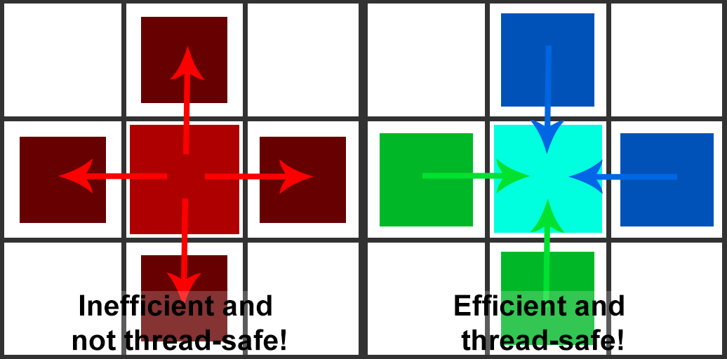
Now, for the propagation itself. I will describe how the distribution would work, not how the gathering would work. This is because it is easier to explain. The code below will show how it works for gathering. This process describes how it works for propagation to one cell. To other cells is the same process with other directions.

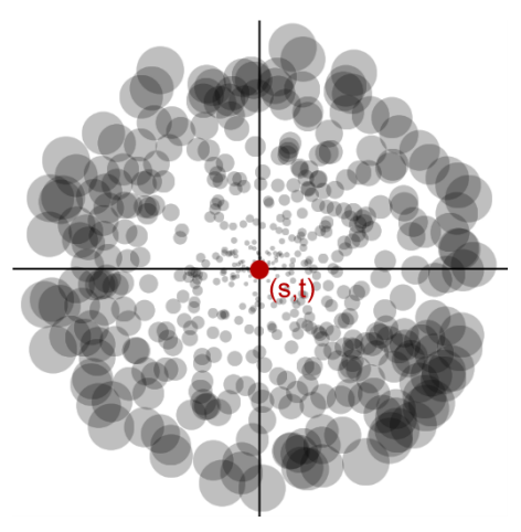
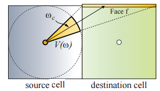
The direction towards the neighbour cell is projected into Spherical Harmonics and evaluated against the stored SH coefficients in the current cell. This cancels out lighting going in other directions. There is a problem with this approach though. We are propagating spherical lighting information through a cubic grid. Try imagining a sphere inside a cube, there are quite some gaps. These gaps will also be visible in the final rendering as unlit spots. The way to fix this is by projecting the light onto the faces of the cell you are propagating it to.

The image below (borrowed from CLPV paper) demonstrates this. The yellow part is the solid angle, which is the part of the sphere used to light, and also what determines how much light is distributed towards a certain face. You need to do this for 5 faces (not the front one, all others) so you cover the entire cube. This preserves directional information (for improved spreading) so results are better lit and you don’t have those ugly unlit spots.

solidangle

The (compute) shader below demonstrates how propagation works in a gathering way, and how the side-faces are used for the accumulation as well.

[code lang=”cpp”]#define LPV_DIM 32
#define LPV_DIMH 16
#define LPV_CELL_SIZE 4.0

int3 getGridPos(float3 worldPos)
{
return (worldPos / LPV_CELL_SIZE) + int3(LPV_DIMH, LPV_DIMH, LPV_DIMH);
}

// https://github.com/mafian89/Light-Propagation-Volumes/blob/master/shaders/lightInject.frag and
// https://github.com/djbozkosz/Light-Propagation-Volumes/blob/master/data/shaders/lpvInjection.cs seem
// to use the same coefficients, which differ from the RSM paper. Due to completeness of their code, I will stick to their solutions.
/*Spherical harmonics coefficients – precomputed*/
#define SH_c0 0.282094792f // 1 / 2sqrt(pi)
#define SH_c1 0.488602512f // sqrt(3/pi) / 2

/*Cosine lobe coeff*/
#define SH_cosLobe_c0 0.886226925f // sqrt(pi)/2
#define SH_cosLobe_c1 1.02332671f // sqrt(pi/3)
#define Pi 3.1415926f

float4 dirToCosineLobe(float3 dir) {
//dir = normalize(dir);
return float4(SH_cosLobe_c0, -SH_cosLobe_c1 * dir.y, SH_cosLobe_c1 * dir.z, -SH_cosLobe_c1 * dir.x);
}

float4 dirToSH(float3 dir) {
return float4(SH_c0, -SH_c1 * dir.y, SH_c1 * dir.z, -SH_c1 * dir.x);
}

// End of common.hlsl.inc

RWTexture3D<float4> lpvR : register(u0);
RWTexture3D<float4> lpvG : register(u1);
RWTexture3D<float4> lpvB : register(u2);

static const float3 directions[] =
{ float3(0,0,1), float3(0,0,-1), float3(1,0,0), float3(-1,0,0) , float3(0,1,0), float3(0,-1,0)};

// With a lot of help from: http://blog.blackhc.net/2010/07/light-propagation-volumes/
// This is a fully functioning LPV implementation

// right up
float2 side[4] = { float2(1.0, 0.0), float2(0.0, 1.0), float2(-1.0, 0.0), float2(0.0, -1.0) };

// orientation = [ right | up | forward ] = [ x | y | z ]
float3 getEvalSideDirection(uint index, float3x3 orientation) {
const float smallComponent = 0.4472135; // 1 / sqrt(5)
const float bigComponent = 0.894427; // 2 / sqrt(5)

const float2 s = side[index];
// *either* x = 0 or y = 0
return mul(orientation, float3(s.x * smallComponent, s.y * smallComponent, bigComponent));
}

float3 getReprojSideDirection(uint index, float3x3 orientation) {
const float2 s = side[index];
return mul(orientation, float3(s.x, s.y, 0));
}

// orientation = [ right | up | forward ] = [ x | y | z ]
float3x3 neighbourOrientations[6] = {
// Z+
float3x3(1, 0, 0,0, 1, 0,0, 0, 1),
// Z-
float3x3(-1, 0, 0,0, 1, 0,0, 0, -1),
// X+
float3x3(0, 0, 1,0, 1, 0,-1, 0, 0
),
// X-
float3x3(0, 0, -1,0, 1, 0,1, 0, 0),
// Y+
float3x3(1, 0, 0,0, 0, 1,0, -1, 0),
// Y-
float3x3(1, 0, 0,0, 0, -1,0, 1, 0)
};

[numthreads(16, 2, 1)]
void main(uint3 dispatchThreadID: SV_DispatchThreadID, uint3 groupThreadID : SV_GroupThreadID)
{
uint3 cellIndex = dispatchThreadID.xyz;

// contribution
float4 cR = (float4)0;
float4 cG = (float4)0;
float4 cB = (float4)0;

for (uint neighbour = 0; neighbour < 6; ++neighbour)
{
float3x3 orientation = neighbourOrientations[neighbour];
// TODO: transpose all orientation matrices and use row indexing instead? ie int3( orientation[2] )
float3 mainDirection = mul(orientation, float3(0, 0, 1));

uint3 neighbourIndex = cellIndex – directions[neighbour];
float4 rCoeffsNeighbour = lpvR[neighbourIndex];
float4 gCoeffsNeighbour = lpvG[neighbourIndex];
float4 bCoeffsNeighbour = lpvB[neighbourIndex];

const float directFaceSubtendedSolidAngle = 0.4006696846f / Pi / 2;
const float sideFaceSubtendedSolidAngle = 0.4234413544f / Pi / 3;

for (uint sideFace = 0; sideFace < 4; ++sideFace)
{
float3 evalDirection = getEvalSideDirection(sideFace, orientation);
float3 reprojDirection = getReprojSideDirection(sideFace, orientation);

float4 reprojDirectionCosineLobeSH = dirToCosineLobe(reprojDirection);
float4 evalDirectionSH = dirToSH(evalDirection);

cR += sideFaceSubtendedSolidAngle * dot(rCoeffsNeighbour, evalDirectionSH) * reprojDirectionCosineLobeSH;
cG += sideFaceSubtendedSolidAngle * dot(gCoeffsNeighbour, evalDirectionSH) * reprojDirectionCosineLobeSH;
cB += sideFaceSubtendedSolidAngle * dot(bCoeffsNeighbour, evalDirectionSH) * reprojDirectionCosineLobeSH;
}

float3 curDir = directions[neighbour];
float4 curCosLobe = dirToCosineLobe(curDir);
float4 curDirSH = dirToSH(curDir);

int3 neighbourCellIndex = (int3)cellIndex + (int3)curDir;

cR += directFaceSubtendedSolidAngle * max(0.0f, dot(rCoeffsNeighbour, curDirSH)) * curCosLobe;
cG += directFaceSubtendedSolidAngle * max(0.0f, dot(gCoeffsNeighbour, curDirSH)) * curCosLobe;
cB += directFaceSubtendedSolidAngle * max(0.0f, dot(bCoeffsNeighbour, curDirSH)) * curCosLobe;
}

lpvR[dispatchThreadID.xyz] += cR;
lpvG[dispatchThreadID.xyz] += cG;
lpvB[dispatchThreadID.xyz] += cB;
}[/code]

Rendering

Rendering is pretty straight forward. You use the G-Buffer’s world space position to get a grid position. If you have those positions as floats, you can easily do trilinear sampling on the three 3D textures used for LPV. With that sampling result you have a set of Spherical Harmonics and you project the world space normal from the G-Buffer into SH and do dot products against the three textures to get scalar values per color component. Multiply that by the albedo and the Ambient Occlusion factor and you have indirect lighting.

The pixel shader below demonstrates this. This is done by rendering a full screen quad and evaluating all pixels. If you have occlusion culling, you can optimize the indirect light rendering by adding it in the G-Buffer phase in a light accumulation buffer, but in my implementation I have a lot of overdraw and no early-Z/occlusion culling.

[code lang=”cpp”]
<pre>// Start of common.hlsl.inc
#define LPV_DIM 32
#define LPV_DIMH 16
#define LPV_CELL_SIZE 4.0

int3 getGridPos(float3 worldPos)
{
return (worldPos / LPV_CELL_SIZE) + int3(LPV_DIMH, LPV_DIMH, LPV_DIMH);
}
float3 getGridPosAsFloat(float3 worldPos)
{
return (worldPos / LPV_CELL_SIZE) + float3(LPV_DIMH, LPV_DIMH, LPV_DIMH);
}

// https://github.com/mafian89/Light-Propagation-Volumes/blob/master/shaders/lightInject.frag and
// https://github.com/djbozkosz/Light-Propagation-Volumes/blob/master/data/shaders/lpvInjection.cs seem
// to use the same coefficients, which differ from the RSM paper. Due to completeness of their code, I will stick to their solutions.
/*Spherical harmonics coefficients – precomputed*/
#define SH_C0 0.282094792f // 1 / 2sqrt(pi)
#define SH_C1 0.488602512f // sqrt(3/pi) / 2

/*Cosine lobe coeff*/
#define SH_cosLobe_C0 0.886226925f // sqrt(pi)/2
#define SH_cosLobe_C1 1.02332671f // sqrt(pi/3)
#define PI 3.1415926f

float4 dirToCosineLobe(float3 dir) {
//dir = normalize(dir);
return float4(SH_cosLobe_C0, -SH_cosLobe_C1 * dir.y, SH_cosLobe_C1 * dir.z, -SH_cosLobe_C1 * dir.x);
}

float4 dirToSH(float3 dir) {
return float4(SH_C0, -SH_C1 * dir.y, SH_C1 * dir.z, -SH_C1 * dir.x);
}

// End of common.hlsl.inc

struct PSIn
{
float4 pos : SV_POSITION;
float3 normal : NORMAL;
float3 tangent : TANGENT;
float3 bitangent : BITANGENT;
float2 texcoord : TEXCOORD0;
float3 posWS : POSITION;
};

sampler trilinearSampler : register(s0);
Texture3D lpvR : register(t0);
Texture3D lpvG: register(t1);
Texture3D lpvB : register(t2);
Texture2D wsPosMap : register(t3);
Texture2D wsNorMap : register(t4);
Texture2D albedoMap : register(t5);
Texture2D ambientOcclusionMap : register(t6);

float4 main(PSIn IN) : SV_Target
{

float3 albedo = albedoMap.Sample(trilinearSampler, IN.texcoord).xyz;
float3 pxPosWS = wsPosMap.Sample(trilinearSampler, IN.texcoord).xyz;
float3 pxNorWS = wsNorMap.Sample(trilinearSampler, IN.texcoord).xyz;
float3 gridPos = getGridPosAsFloat(pxPosWS);

// https://github.com/mafian89/Light-Propagation-Volumes/blob/master/shaders/basicShader.frag
float4 SHintensity = dirToSH(-pxNorWS);
float3 lpvIntensity = (float3)0;

float4 lpvRtex = lpvR.SampleLevel(trilinearSampler, gridPos / float3(LPV_DIM, LPV_DIM, LPV_DIM), 0);
float4 lpvGtex = lpvG.SampleLevel(trilinearSampler, gridPos / float3(LPV_DIM, LPV_DIM, LPV_DIM), 0);
float4 lpvBtex = lpvB.SampleLevel(trilinearSampler, gridPos / float3(LPV_DIM, LPV_DIM, LPV_DIM), 0);

lpvIntensity = float3(
dot(SHintensity, lpvRtex),
dot(SHintensity, lpvGtex),
dot(SHintensity, lpvBtex));

float3 finalLPVRadiance = max(0, lpvIntensity) / PI;

float4 result = float4(finalLPVRadiance, 1.0) * ambientOcclusionMap.Load(int3(IN.pos.xy, 0)).r * float4(albedo, 1.0);
return result;
}</pre>
[/code]

Pros and cons

This algorithm, like any other, has its pros and cons.

Pros

  • The algorithm is very fast
  • One data structure which can support multiple lights
  • Completely dynamic and real-time

Cons

  • The amount of SH coefficients used (4) has only about 75% accuracy. This means more objects will get incorrect lighting and light bleeding will happen in wrong places.
  • Trade-off between more local reflections or more global reflection as the size of the grid influences this. Can be solved by using Cascaded LPVs.
  • Does not allow for specular reflections. Can be added with Screen-Spaced Reflections.
  • Only allows for one light bounce. There are workarounds, but that also has its tradeoffs.

Resources

Spherical Harmonics papers and posts:

Reflective Shadow Maps: Part 2 – The implementation

I managed to implement a very naive version of Reflective Shadow Maps (an algorithm described in this paper). This post will explain how I did that and what the pitfalls were. It will also cover some possible optimizations.

rsm_impl

Figure 1: From left to right: Render without Reflective Shadow Maps, render with reflective shadow maps, difference

The result

In figure 1 you see one of the results produced by RSM. The images you see use the Stanford Bunny and three differently colored quads. In the left image, you see the result of a render without RSM, using just a spot light. Whatever falls in the shadow is completely black. In the middle image you see the same image, but rendered using RSM. Notable differences are the brighter colors everywhere, the pink color bleeding onto the floor and the bunny, the shadow not being completely black. The last image shows the differene between the two images, thus what RSM contributed to the image. You might see some harder edges and artifacts in the middle and righter image, but that can be solved by tweaking the sample kernel size, indirect light intensity, and the amount of samples taken.

The implementation

The engine I implemented this algorithm in has a cross-platform rendering architecture allowing us to create rendering techniques (like deferred shading, shadow mapping, etc.) that will theoretically work on any platform we support. The architecture was set up to be multi-threading compatible and as stateless as possible. It also uses a lot of terminology found in DirectX 11 and 12. The shaders were written in HLSL and the renders made with DirectX 11. Keep this in mind when I talk about implementation details.

I had already set up a deferred renderer with shadow maps for directional lights prior to writing this article. Then I implemented RSM for directional lights. After that, I added spot light shadow maps and added support for RSM to them.

Expanding the shadow map

Traditionally, Shadow Maps (SM) are no more than a depth map. This means you don’t even need a pixel/fragment shader for filling an SM. However, for RSM, you need a few extra buffers. You need to store the world space positions, world space normals, and the flux. This means you need multiple render targets and a pixel/fragment shader to fill them. Keep in mind that you need to cull back faces instead of front faces for this technique. Using front face culling is a commonly used technique to avoid shadow artifacts, but this does not work with RSM.

You pass the world space normal and position to the pixel shader and pass those through to the corresponding buffers. If you have normal mapping, you calculate that in the pixel shader as well. The flux is calculated in the pixel shaders and is the albedo of the material multiplied by the light’s color. For spot lights, you multiply this by the falloff. For directional lights, this will simply look like an unshaded image.

Preparing the shading pass

For the shading pass, you need to do a few things. You need to bind all buffers used in the shadow pass as textures. You also need random numbers. The paper tells you to precalculate those numbers and store them into a buffer in order to save operations for the sampling pass. Since the algorithm is heavy in terms of performance, I thoroughly agree with the paper. They also recommend this to have temporal coherency. This means it will avoid flickering images when every frame uses different shadows.

You need two random floats in the [0, 1] range per sample you take. These random numbers will be used to determine the coordinates of a sample. You will also need the same matrix you use transform world space positions to shadow map texture space positions. Further than that, a non-comparison sampler that clamps with black border colors will also be necessary.

Performing the shading pass

This is the hard part, especially to get it right. I recommend doing the indirect shading pass after you have done the direct shading for a particular light. This is because you need a full screen quad to do this and this works fine for directional lights. However, for spot and point lights you generally want to use shaped meshes with some form of culling to fill less pixels.

I will show a piece of code below that calculates the indirect shading per pixel. After that, I will step through the code and explain what is happening.

[code language=”cpp”]float3 DoReflectiveShadowMapping(float3 P, bool divideByW, float3 N)
{
float4 textureSpacePosition = mul(lightViewProjectionTextureMatrix, float4(P, 1.0));
if (divideByW) textureSpacePosition.xyz /= textureSpacePosition.w;

float3 indirectIllumination = float3(0, 0, 0);
float rMax = rsmRMax;

for (uint i = 0; i < rsmSampleCount; ++i)
{
float2 rnd = rsmSamples[i].xy;

float2 coords = textureSpacePosition.xy + rMax * rnd;

float3 vplPositionWS = g_rsmPositionWsMap.Sample(g_clampedSampler, coords.xy).xyz;
float3 vplNormalWS = g_rsmNormalWsMap.Sample(g_clampedSampler, coords.xy).xyz;
float3 flux = g_rsmFluxMap.Sample(g_clampedSampler, coords.xy).xyz;

float3 result = flux
* ((max(0, dot(vplNormalWS, P – vplPositionWS))
* max(0, dot(N, vplPositionWS – P)))
/ pow(length(P – vplPositionWS), 4));

result *= rnd.x * rnd.x;
indirectIllumination += result;
}
return saturate(indirectIllumination * rsmIntensity);
}[/code]

The first argument in the function is P, which is the world space position for a specific pixel. DivideByW is used for the perspective divide required to get a correct Z value. N is the world space normal at a pixel.

[code language=”cpp”]
float4 textureSpacePosition = mul(lightViewProjectionTextureMatrix, float4(P, 1.0));
if (divideByW) textureSpacePosition.xyz /= textureSpacePosition.w;

float3 indirectIllumination = float3(0, 0, 0);
float rMax = rsmRMax;
[/code]

This section sets up the texture space position, initializes the indirect lighting contribution where samples will accumulate into, and set the rMax variable found in the lighting equation in the paper which I will cover in the next section. Basically, rMax is the maximum distance the random sample can be from the texture space position.

[code language=”cpp”]
for (uint i = 0; i < rsmSampleCount; ++i)
{
float2 rnd = rsmSamples[i].xy;

float2 coords = textureSpacePosition.xy + rMax * rnd;

float3 vplPositionWS = g_rsmPositionWsMap.Sample(g_clampedSampler, coords.xy).xyz;
float3 vplNormalWS = g_rsmNormalWsMap.Sample(g_clampedSampler, coords.xy).xyz;
float3 flux = g_rsmFluxMap.Sample(g_clampedSampler, coords.xy).xyz;
[/code]

Here we open the loop and prepare our variables for the equation. In order to optimize it a bit further, the random samples that I calculated are already coordinate offsets, meaning I only have to add rMax * rnd to the texture space coordinates to get my UV coordinates. If the UV coordinates fall outside of the [0,1] range, the samples will be black. Which is logical, since it falls outside of the light’s range, thus does not have any shadow map point to sample from.

[code language=”cpp”]
float3 result = flux
* ((max(0, dot(vplNormalWS, P – vplPositionWS))
* max(0, dot(N, vplPositionWS – P)))
/ pow(length(P – vplPositionWS), 4));

result *= rnd.x * rnd.x;
indirectIllumination += result;
}
return saturate(indirectIllumination * rsmIntensity);
[/code]

This is the part where the indirect lighting equation (displayed in figure 2) is evaluated and weighted by the distance between the point and the pixel light. The equation looks daunting and the code doesn’t really tell you what’s going on either, so I will explain. The variable Φ (phi) is the flux, which is the radiant intensity. The previous article describes this in more detail.

The flux (Φ) is scaled by two dot products. The first dot product is between the pixel light normal and the direction from the pixel light to the surface point. The second dot product is between the surface normal and the direction from the surface point to pixel light. In order to not get inverted light contributions, those dot products are clamped between [0, ∞]. In this equation they do the normalization step last, I assume for performance reasons. It is equally valid to normalize the directions before doing the dot products.

equation
Figure 2: The equation for irradiance at a point in space by pixel light
p

The result from this shader pass can be blended on a backbuffer and will give results as seen in figure 1.

Pitfalls

While implementing this algorithm, I ran into some issues. I will cover these issues to avoid people from making the same mistakes.

Incorrect sampler

I spent a considerable amount of time figuring out why my indirect light seemed to repeat itself. Crytek’s Sponza does not have their UV coordinates in the [0,1] range, so we needed a sampler which wrapped. This is however a horrible property when you are sampling from (reflective) shadow maps.

Tweakable values

To improve my workflow, it was vital to have some variables tunable at the touch of a button. I can increase the intensity of the indirect lighting and the sampling range (rMax). For reflective shadow mapping, these variables should be tweakable per light. If you sample in a big range, you get lighting from everywhere, which is useful for big scenes. For more local indirect lighting, you will need a smaller range. Figure 3 shows global and local indirect lighting.

rMax
Figure 3: Demonstration of rMax sensitivity.  

Separate pass

Initially I thought I could do the indirect lighting in the shader that does the light gathering for deferred rendering. For directional lights, this works, because you render a full screen quad anyway. However, for spot- and pointlights, you try to minimize the fill rate. I decided to move the indirect lighting to a separate pass, something that is necessary if you want to do the screen space interpolation as wel.

Cache inefficient by nature

The algorithm is horribly cache inefficient. The algorithm samples randomly around a point in multiple textures. The  amount of samples taken without optimization is unacceptably high as well. With a resolution of 1280 * 720 and a sample count of 400 you take 1.105.920.000 samples per light.

Pros & cons

I will list the pros and cons of this indirect lighting algorithm that I have encountered. I do not have a lot to compare it to, since this is the first that I am implementing.

Pros Cons
Easy to understand algorithm Very cache inefficient
Integrates neatly with a deferred renderer Requires tweaking of variables
Can be used in other algorithms (LPV) Forced choice between local and global indirect light

Optimizations

I have made some attempts to increase the speed of this algorithm. As they discuss in the paper (link at the top of this page) they perform a screen space interpolation. I got this to work and it sped up the rendering quite a bit. Below I will describe what I have done and make a comparison (in frames per second) between the following states using my 3-walls-with-bunny scene; no RSM, naïve RSM, and interpolated RSM .

Z-check

One reason why my RSM was underperforming was because I was also testing for the pixels that were part of the skybox. A skybox definitely does not need indirect lighting. The speedup this gives depends on how much of the skybox you would actually see.

Pre-calculating random samples on the CPU

Pre-calculating the random samples not only gives you more temporal coherency, it also saves you from having to regenerate those samples in the shaders.

Screen space interpolation

The article proposes to use a low resolution render target for evaluating the indirect lighting. For scenes with a lot of smooth normals and straight walls, lighting information can easily be interpolated between lower resolution points. I am not going to describe this interpolation in detail, to keep this article a bit shorter.

Results and conclusion

Below are my results for a few different sample counts. I have a few observations on these results.

  • Logically, the FPS stays around 700 for different sample counts when there is no RSM calculation done.
  • Interpolation brings some overhead and becomes less useful with low sample counts.
  • Even with 100 samples, the resulting image looked pretty good. This might be due to the interpolation which is “blurring” the indirect light. This makes it look more diffuse.
Sample count FPS for No RSM FPS for Naive RSM FPS for Interpolated RSM
100 ~700 152 264
200 ~700 89 179
300 ~700 62 138
400 ~700 44 116

Reflective Shadow Maps

Reflective Shadow Maps (RSM) is an algorithm that extends “simple” Shadow Maps. The algorithm allows for a single diffuse light bounce. This means that, besides direct illumination, you get indirect illumination. This article breaks down the algorithm from the paper to explain it in a more human-friendly way. I will also briefly cover Shadow Mapping.

Shadow Mapping

Shadow Mapping (SM) is a shadow generation algorithm. This algorithm stores the distance from a light to an object in a depth map. Figure 1 shows an example of a depth map. It stores the distance (depth) per pixel. So, when you have a depth map from a light’s point of view, you then draw the scene from the camera’s point of view. To determine if an object is lit, you check the distance from the light to that object. If the distance to the object is greater than what is stored in the shadow (depth) map, the object is in the shadow. This means the object must not be lit. Figure 2 shows an example. You do these checks per pixel.

5394470202_309d6fe655

Figure 1: This image shows a depth map. The closer the pixel is, the brighter it appears.
shadowmapexample

Figure 2: The distance from the light to the pixel in the shadow is greater than the distance stored in the depth map.

Reflective Shadow Mapping

Now that you understand the basic concept of Shadow Mapping, we continue with Reflective Shadow Mapping (RSM). This algorithm extends the functionality of “simple” Shadow Maps. Besides depth data, you also store world space coordinates,the world space normals, and the flux. I will explain why you store these pieces of data.

The data

World space coordinates

You store the world space coordinates in a Reflective Shadow Map to determine the world space distance between pixels. This is useful for calculating light attenuation. Light attenuates (becomes less concentrated) based on the distance it travels. The distance between two points in space are used to calculate how intense the lighting is.

Normals

The (world space) normal is used to calculate the light bouncing off of a surface. In case of the RSM, it is also used to determine the validity of the pixel as a light for another pixel. If two normals are very similar, they will not contribute much bouncing light for each other.

(Luminous) Flux

Flux is the luminous intensity of a light source. The unit of measurement for this is Lumen, a term you see on light bulb packages nowadays. The algorithm stores the flux for every pixel checked while drawing the shadow map. Flux is calculated by multiplying the reflected light intensity by a reflection coefficient. For directional lights, this would give a uniformly lit image. For spot lights, you take the angle falloff into consideration. Attenuation and receiver cosine are  left out of this calculation, because this is taken into account when you calculate the indirect lighting. The article does not go into detail about this. Figure 3 shows an image from the RSM paper displaying the flux for a spot light in the fourth image.

rsm_maps

Figure 3: This image shows the four maps contained in an RSM. From left to right; depth map, world space coordinates, world space normals, flux

Applying the data

Now that we have generated the data (theoretically), it is time to apply it to a final image. When you draw the final image, you test all lights for every pixel. Besides just lighting the pixels using the lights, you now also use the Reflective Shadow Map.

A naive approach to calculating the light contribution is to test all texels in the RSM. You check if the normal of the texel in the RSM is not pointing away from the pixel you are evaluating. This is done using the world space coordinates and the world space normals. You calculate the direction from the RSM texel’s world space coordinates to that of the pixel. You then compare that to the direction the normal is pointing to, using the vector dot product. Any positive value means the pixel should be lit by the flux stored in the RSM. Figure 4 demonstrates this algorithm.

indirect_lighting

Figure 4: Demonstration of indirect light contribution based on world space positions and normals

Shadow maps (and RSMs) are large by nature (512×512=262144 pixels), so doing a test for every texel is far from optimal. Instead, it is best to take a set amount of samples from the map. The amount of samples you take depends on how powerful your hardware is. An insufficient amount of samples might give artifacts like banding or flickering colors.

The texels that will contribute most to the lighting result are the ones closest to the pixel you are evaluating. A sampling pattern that takes the most samples near the pixel’s coordinates will give the best results. The paper describes that the sampling density decreases with the squared distance from the pixel we are testing. They achieve this by converting the texture coordinates to polar coordinates relative to the point we are testing.

Since we are doing “importance sampling” here, we need to scale the intensity of the samples by a factor related to the distance. This is because samples that are further away get sampled less often, but would in reality still contribute the same amount of flux. Samples closer by get sampled more often, but samples farther away are more intense. This evens out an inequality while keeping the sample count low. Figure 5 shows how this works.

importance_sampling

Figure 5: Importance sampling. More samples are taken from the center and samples are scaled by a factor related to their distance from the center point. Borrowed from the RSM paper.

When you have a sample, you treat that sample the same as you would treat a point light. You use the flux value as the light’s color and only light objects in front of this sample.

The paper goes into more detail on how to further optimize this algorithm, but I will stop here. The section on Screen-Space Interpolation describes how you can gain more speed, but for now  I think importance sampling will suffice. I am glad to say that I understand the RSM algorithm enough to build an implementation in C++/DirectX11. I will do my best to answer any questions you may have.

Lots of balls

A new week, a new assignment. This week I get to optimize a piece of code that renders a “glass” ball on a background, letting through some of the color hidden in the background image. Puzzling on my own and talking to classmates helped in creating code which I couldn’t get any faster. I’ve learned a lot doing this and discussing it with peers.

The initial code draws a colorful landscape with a black & white overdraw on it, making it a greyscale and darker image. The ball samples pixels from the colorful version of the image. The goal of this week’s assignment is to optimize using several rules of thumb, “Get rid of expensive operations”, “Precalculate”, “Use the power of 2”, “Avoid conditional jumps”, and “Get out early”. High-level optimizations were not specifically required, but makes the code a lot faster. I will show both versions of “Game.cpp”, mine and the unoptimized one.

glassbal
This is how the glass-ball effect looks.

The initial code was written by my teacher, Jacco Bikker, for the NHTV, and is intended to be optimized. The most relevant bit is in the “Game.cpp” and is as follows.
[code language=”cpp”]#include "game.h"
#include "surface.h"

using namespace Tmpl8;

// ———————————————————–
// Scale a color (range: 0..128, where 128 is 100%)
// ———————————————————–
inline unsigned int ScaleColor( unsigned int orig, char scale )
{
const Pixel rb = ((scale * (orig & ((255 << 16) + 255))) >> 7) & ((255 << 16) + 255);
const Pixel g = ((scale * (orig & (255 << 8))) >> 7) & (255 << 8);
return (Pixel)rb + g;
}

// ———————————————————–
// Draw a glass ball using fake reflection & refraction
// ———————————————————–
void Game::DrawBall( int bx, int by )
{
Pixel* dst = m_Surface->GetBuffer() + bx + by * m_Surface->GetPitch();
Pixel* src = m_Image->GetBuffer();
for ( int x = 0; x < 128; x++ )
{
for ( int y = 0; y < 128; y++ )
{
float dx = (float)(x – 64);
float dy = (float)(y – 64);
int dist = (int)sqrt( dx * dx + dy * dy );
if (dist < 64)
{
int xoffs = (int)((dist / 2 + 10) * sin( (float)(x – 50) / 40.0 ) );
int yoffs = (int)((dist / 2 + 10) * sin( (float)(y – 50) / 40.0 ) );
int u1 = (((bx + x) – 4 * xoffs) + SCRWIDTH) % SCRWIDTH;
int v1 = (((by + y) – 4 * yoffs) + SCRHEIGHT) % SCRHEIGHT;
int u2 = (((bx + x) + 2 * xoffs) + SCRWIDTH) % SCRWIDTH;
int v2 = (((by + y) + 2 * yoffs) + SCRHEIGHT) % SCRHEIGHT;
Pixel refl = src[u1 + v1 * m_Image->GetPitch()];
Pixel refr = src[u2 + v2 * m_Image->GetPitch()];
int reflscale = (int)(63.0f – 0.015f * (1 – dist) * (1 – dist));
int refrscale = (int)(0.015f * (1 – dist) * (1 – dist));
dst[x + y * m_Surface->GetPitch()] =
ScaleColor( refl, 41 – (int)(reflscale * 0.5f) ) + ScaleColor( refr, 63 – refrscale );
float3 L = Normalize( float3( 60, -90, 85 ) );
float3 p = float3( (x – 64) / 64.0f, (y – 64) / 64.0f, 0 );
p.z = sqrt( 1.0f – (p.x * p.x + p.y * p.y) );
float d = min( 1, max( 0, Dot( L, p ) ) );
d = powf( d, 140 );
Pixel highlight = ((int)(d * 255.0f) << 16) + ((int)(d * 255.0f) << 8) + (int)(d * 255.0f);
dst[x + y * m_Surface->GetPitch()] = AddBlend( dst[x + y * m_Surface->GetPitch()], highlight );
}
}
}
}

// ———————————————————–
// Initialize the game
// ———————————————————–
void Game::Init()
{
m_Image = new Surface( "testdata/mountains.png" );
m_BallX = 100;
m_BallY = 100;
m_VX = 1.6f;
m_VY = 0;
}

// ———————————————————–
// Draw the backdrop and make it a bit darker
// ———————————————————–
void Game::DrawBackdrop()
{
m_Image->CopyTo( m_Surface, 0, 0 );
Pixel* src = m_Surface->GetBuffer();
unsigned int count = m_Surface->GetPitch() * m_Surface->GetHeight();
for ( unsigned int i = 0; i < count; i++ )
{
src[i] = ScaleColor( src[i], 20 );
int grey = src[i] & 255;
src[i] = grey + (grey << 8) + (grey << 16);
}
}

// ———————————————————–
// Main game tick function
// ———————————————————–
void Game::Tick( float a_DT )
{
m_Surface->Clear( 0 );
DrawBackdrop();
DrawBall( (int)m_BallX, (int)m_BallY );
m_BallY += m_VY;
m_BallX += m_VX;
m_VY += 0.2f;
if (m_BallY > (SCRHEIGHT – 128))
{
m_BallY = SCRHEIGHT – 128;
m_VY = -0.96f * m_VY;
}
if (m_BallX > (SCRWIDTH – 138))
{
m_BallX = SCRWIDTH – 138;
m_VX = -m_VX;
}
if (m_BallX < 10)
{
m_BallX = 10;
m_VX = -m_VX;
}
}[/code]

I will not dive in too much depth on what the pieces of the code does, but Init runs once, Tick runs every frame, DrawBackdrop draws the dark and grey overlay on top of the bright coloured landscape, which is visible through the ball drawn with DrawBall. The things to optimize will be drawing the background (with currently DrawBackdrop) and DrawBall. I did not pay attention to memory usage, as that isn’t the intention of the excersize. This is the code that I ended up with:
[code language=”cpp”]#include "game.h"
#include "surface.h"
#include <iostream>
#include <time.h>

using namespace Tmpl8;

Surface* imageWithBackdrop;

// ———————————————————–
// Scale a color (range: 0..128, where 128 is 100%)
// ———————————————————–
inline unsigned int ScaleColor( unsigned int orig, int scale )
{
const Pixel rb = ((scale * (orig & ((255 << 16) | 0xFF))) >> 7) & ((255 << 16) + 255);
const Pixel g = ((scale * (orig & (255 << 8))) >> 7) & (255 << 8);
return (Pixel)rb + g;
}

// ———————————————————–
// Draw a glass ball using fake reflection & refraction
// ———————————————————–
const float3 L = Normalize(float3(60, -90, 85));
unsigned int imageWidth;
unsigned int imageHeight;
int distances[128 * 128];
Pixel highlights[128 * 128];
int xOffs[128 * 128];
int yOffs[128 * 128];
int reflScales[128 * 128];
int refrScales[128 * 128];
const static int pitch = SCRWIDTH;

#define BALLS 100

struct Ball
{
float m_X, m_Y, m_VX, m_VY;
};
Ball balls[BALLS];

void Game::DrawBall( int bx, int by )
{
static Pixel* src = m_Image->GetBuffer();
Pixel* dst = m_Surface->GetBuffer() + bx + by * m_Surface->GetPitch();

for (int y = 0; y < 128; ++y )
{
for ( int x = 0; x < 128; ++x )
{
unsigned int index = (y << 7) + x;

if (distances[index] < 64)
{
unsigned int u1 = ((((bx + x) – (xOffs[index] << 1)) + imageWidth) << 22) >> 22;
unsigned int v1 = ((((by + y) – (yOffs[index] << 1)) + imageHeight) << 22) >> 12;
unsigned int u2 = (((bx + x) + xOffs[index] + imageWidth) << 22) >> 22;
unsigned int v2 = (((by + y) + yOffs[index] + imageHeight) << 22) >> 12;

Pixel refl = src[u1 + v1]; //Reflection
Pixel refr = src[u2 + v2]; //Refraction

dst[x + y * pitch] =
AddBlend(
ScaleColor(refl, reflScales[index]) + ScaleColor(refr, refrScales[index]),
highlights[index]
);
}
}
}
}

// ———————————————————–
// Draw the backdrop and make it a bit darker
// ———————————————————–
void Game::DrawBackdrop()
{
m_Image->CopyTo(m_Surface, 0, 0);
Pixel* src = m_Surface->GetBuffer();
unsigned int count = m_Surface->GetPitch() * m_Surface->GetHeight();
for (unsigned int i = 0; i < count; i++)
{
src[i] = ScaleColor(src[i], 20);
int grey = src[i] & 255;
src[i] = grey + (grey << 8) + (grey << 16);
}
}

void DrawBackground(Surface* a_Target)
{
memcpy(a_Target->GetBuffer(), imageWithBackdrop->GetBuffer(),
imageWithBackdrop->GetPitch() * imageWithBackdrop->GetHeight() * sizeof(Pixel));
}

// ———————————————————–
// Initialize the game
// ———————————————————–
#define TEST_ITERATIONS 512
void Game::Init()
{
srand((unsigned int)time(0));
m_Image = new Surface("testdata/mountains.png");
imageWidth = m_Image->GetWidth();
imageHeight = m_Image->GetHeight();

for (int y = 0; y < 128; y++)
{
float dy = (float)(y – 64);
for (int x = 0; x < 128; x++)
{
float dx = (float)(x – 64);
int dist = (int)sqrt(dx * dx + dy * dy);
distances[y * 128 + x] = dist;
}
}

for(int y = 0; y < 128; y++)
{
int dy = y – 64;
float pY = dy / 64.0f;

for (int x = 0; x < 128; x++)
{
xOffs[y * 128 + x] = (int)(((distances[y * 128 + x] >> 1) + 10) * sin((x – 50) / 40.0f));
xOffs[y * 128 + x] <<= 1;
yOffs[y * 128 + x] = (int)(((distances[y * 128 + x] >> 1) + 10) * sin((y – 50) / 40.0f));
yOffs[y * 128 + x] <<= 1;

reflScales[y * 128 + x] = (int)(63.0f – 0.015f * (1 – distances[y * 128 + x]) * (1 – distances[y * 128 + x]));
reflScales[y * 128 + x] = 41 – (reflScales[y * 128 + x] >> 1);
refrScales[y * 128 + x] = (int)(0.015f * (1 – distances[y * 128 + x]) * (1 – distances[y * 128 + x]));
refrScales[y * 128 + x] = 63 – refrScales[y * 128 + x];

float3 p((x – 64) / 64.0f, pY, 0);
p.z = sqrt(1.0f – (p.x * p.x + p.y * p.y));

float d = Dot(L, p);
if (d > 0.96f) //Approximate value, anything below this doesn’t affect the highlight.
{
d = min(1, max(0, d));
d = pow(d, 140);
auto di = (int)(d * 255.0f);
Pixel highlight = (di << 16) + (di << 8) + di;

highlights[y * 128 + x] = highlight;
}
else
{
highlights[y * 128 + x] = 0;
}
}
}

for (int i = 0; i < BALLS; i++)
{
balls[i].m_X = (float)(80 + rand()%(SCRWIDTH-230));
balls[i].m_Y = (float)(16 + rand() % (SCRHEIGHT – 230));
balls[i].m_VX = 1.6f;
balls[i].m_VY = 0;
}

DrawBackdrop();
imageWithBackdrop = new Surface(m_Surface->GetPitch(), m_Surface->GetHeight());
memcpy(imageWithBackdrop->GetBuffer(), m_Surface->GetBuffer(),
m_Surface->GetPitch() * m_Surface->GetHeight() * sizeof(Pixel));

unsigned long long timings[TEST_ITERATIONS];
for (int iterations = 0; iterations < TEST_ITERATIONS; iterations++)
{
TimerRDTSC timer;
timer.Start();
DrawBall(300, 300);
timer.Stop();
timings[iterations] = timer.Interval();
}
unsigned long long total = 0;
for (int i = 0; i < TEST_ITERATIONS; i++)
{
total += timings[i];
}
total /= TEST_ITERATIONS;
std::cout << total << " is average for DrawBall\n";
TimerRDTSC timer;
timer.Start();
DrawBackground(m_Surface);
timer.Stop();
std::cout << timer.Interval() << std::endl;
}

// ———————————————————–
// Main game tick function
// ———————————————————–
void Game::Tick( float a_DT )
{
DrawBackground(m_Surface);

for (int i = 0; i < BALLS; i++)
{
DrawBall((int)balls[i].m_X, (int)balls[i].m_Y);
balls[i].m_X += balls[i].m_VX;
balls[i].m_Y += balls[i].m_VY;
balls[i].m_VY += 0.2f;
if (balls[i].m_Y >(SCRHEIGHT – 128))
{
balls[i].m_Y = SCRHEIGHT – 128;
balls[i].m_VY = -0.96f * balls[i].m_VY;
}
if (balls[i].m_X > (SCRWIDTH – 138))
{
balls[i].m_X = SCRWIDTH – 138;
balls[i].m_VX = -balls[i].m_VX;
}
if (balls[i].m_X < 10)
{
balls[i].m_X = 10;
balls[i].m_VX = -balls[i].m_VX;
}
}
}[/code]

Background

I started off with the background, which was rendering slow due to the DrawBackdrop every frame. The background image never changes, which means drawing the backdrop only once on a copy of the landscape and then drawing that pre-rendered surface as background would save me quite some cycles. I moved the call to DrawBackdrop to the Init-function and drew that to a new surface.

This saved me a lot of cycles. The cycles on itself don’t say a lot, but in comparison to optimized results, they do. Going from 100 to 10 cycles would be 10 times faster, while 100 itself doesn’t give any valuable information away. The rendering of the background with the backdrop costed me about 1871784 cycles on average (on 10 tests). The optimized DrawBackground, using the pre-rendered surface and memcpy, uses roughly 285000 cycles on average (on 512 tests). This is about 15.2% of the unoptimized version. Clearing the screen wasn’t necessary, so that line is removed in the final code.

The Ball

For the optimizations performed on drawing the ball, I will discuss the before mentioned topics. The original code uses 4912748 cycles on average for 512 tests. The optimized version uses about 433500 on average, with 512 tests. That means there’s only 8.8% left of the cost!

Get rid of expensive operations (and use the power of 2)

The original code uses a lot of expensive operations. Most of that stuff can be precalculated, which is what I went for. I did try some other ideas before I started to move those calculations to the Init function. Here’s a short list of things I’ve figured out, some with help of my classmates.

  • Changing “powf” to “pow” gives an enormous reduction in cycles. This is because “pow” takes an integer as power and “powf” takes a float, which is a lot harder to calculate. Since the input is 140, it could just be an integer.
  • Reducing the calls to “pow” increases performance a lot. “pow” is still quite expensive, so we’d want to reduce its use as much as we can. The code using “pow” draws a specular highlight on the ball, but that’s just a small dot. Doing “pow” for every pixel while only about 5% should need it is a waste. I approximated a number of about 0.96 (depending on the power), where every result of the Dot-product higher than that will draw a pixel for the specular highlight. 96% less calls to “pow” is great.
  • The distance calculations were faster with floats. I didn’t expect this, since integer operations are practically always faster. But, I read somewhere that the compiler might use SIMD to optimize floating-point operations, making it a lot faster. This is why you should always test and record, instead of blindly changing code which you think might run faster.
  • Modulo is slow. It can be used to have looping textures, but the operation is slow. The original code used modulo on the window width, but it sampled colours (for refraction and reflection) from the image provided with the project. The fortunate thing is that the background image has a dimension of 1024×640. Since 1024 is a power of 2, you can use a logical and operator (&) to scrape off the bits not included in the 1024-range, making it wrap neatly. This speeds up the code enormously, since it saves two modulo calls per pixel per ball. The height isn’t a power of two, but we can adjust the image to make it so. Using PhotoShop, I padded the height to 1024, repeating the image for sampling purposes. Now I can do the same thing with the height, removing all uses of modulo.
  • Bitshifting is faster than logical and (&). In the previous list item, I removed the modulo calls, by replacing them with logical ands, greatly increasing speed. But, since we’re only using the first 10 bits, we can shift 22 bits to the left, truncating all those bits and then shifting them back to get the wrapped value between 0 and 1023. This saved several thousand cycles on average.
  • int-float conversions are slow. “(int)(reflscale * 0.5f)” converts “reflscale” to a float to do the multiplication and then converts that back to an int. Since 0.5 is a reciprocal of a power of 2, we can just use a bitshift to divide the number by 2. “reflscale >> 1” does the job perfectly and is a lot faster.

Precalculate

Precalculating most stuff was what gave the biggest improvements in cycle reduction. I’ve moved almost everything, apart from the sampling from the background, to the Init functions and made it accessible by array indices.

I started precalculating stuff when I noticed the “sin()” calls always used a number of 0 to 128 as arguments. I created an array of precalculated sines and referenced to that, giving a great boost in speed. I wanted to do the same for the distances, using an array of 64×64, because the distances are the same for all quadrants of the circle. This gave me an off-by-one error, making the code draw 2 unwanted lines. Since memory usage wasn’t the focus, I figured I could just use 128×128 arrays for the calculations, avoiding calls to “abs()”.

After this, I sat down with a classmate, talking about which optimizations we used and soon figured out that practically everything can be cached quite easily. The entire specular highlight can be saved in an array, getting rid of “sqrt()”-calls, “pow”-calls, “sin()”-calls, and floats in the rendering of each ball every frame. The highlight-array is basically just an overlay for the ball, blended with “AddBlend()”. All the heavy code is now in the Init-function, basically leaving only integer arithmetic, sampling from an image, blending, and bitshifting in the DrawBall-function. Pre-rendering every possible position for a ball could also be a solution, but having 800×600 pre-rendered balls in memory isn’t a neat solution in my opinion.

Avoid conditional jumps

Unrolling my loops would probably speed things up, but I read that the compiler unrolls the loops automatically. An old forum post a user states that the Visual C++ compiler unwinds loops where possible to increase performance. My project settings are set to produce the fastest code (opposed to the smaller code option).

Get out early

The “Get out early”-principle basically means to break the loop if the rest of the iterations aren’t helpful anymore. I tested code which broke the X-loop after it drew the last pixel of that row. Unfortunately, the checks for these last pixels increased the amount of cycles more than it saved, which is why I don’t break the loop.

Conclusion

The core of this optimization challenge was precalculation (caching) and getting rid of expensive function calls. I got the ball to render more than 10 times as fast and I can run the program drawing 100 balls on screen with over 30 FPS on my laptop. I’m happy with the result, yet it frustrates me a little bit that I can’t find anything else in that piece of code to optimize, but I guess I’ll learn more ways to do that in future lectures. Thanks for reading!

Getting things sorted

For an assignment for Programming 3 at IGAD, I have to optimize a piece of code. The code transforms, sorts, and renders an amount of sprites. Optimization of the rendering was done in class, so the sorting is the biggest bottleneck at the moment. Which is what I will dedicate this post to. I’ve found some sorting algorithms that I think are very interesting. The ones I will talk about are QuickSort, Radix Sort, and Tree Sort. The algorithm used in the code at first is an unoptimized Bubble Sort, which is very slow.

The sorting algorithm will have to deal with a high amount of sprites to sort, based on their Z-value, which is a floating-point number. The amount of sprites ranges is at least above 5000 and the assignment is to make the code render as many sprites on screen as I can.

Tree Sort

The first decent algorithm I imagined without research was a tree structure, where you would put all data in a binary tree. This automatically sorts the tree, which you could flatten back to an array quite easily. Apparently, this exists and isn’t a terrible solution for sorting. The only problem you face is when you have an unbalanced tree. If you have the maximum value as a first value, anything that gets added will get added to the left child nodes. With a bit of bad luck, this could be the case for a lot of elements, making you traverse every element before adding a new one.

The ease of implementation is what would make this an option for the simulation that I have to optimize. I will not use this one, but I will give example pseudo-code of how I would implement it. It can probably optimized in really simple ways, but since I’m not using this algorithm, I see no need in working on that at the moment. Adding to the tree would be as follows.

[code language=”cpp”]struct TreeNode
{
/*
* I’m using float3-vectors, this could be a Sprite as well.
* The code just draws sprites at positions.
*/
float3 value;
TreeNode* leftNode;
TreeNode* rightNode;

TreeNode(float3 a_value)
: value(a_value), leftNode(nullptr), rightNode(nullptr){}

~TreeNode()
{
if(leftNode) delete leftNode;
if(rightNode) delete rightNode;
}

void Insert(float3& a_other)
{
if(a_other.z <= value.z)
{
if(leftNode == nullptr)
leftNode = new TreeNode(a_other);
else
leftNode->Insert(a_other);
}
else
{
if(rightNode == nullptr)
rightNode = new TreeNode(a_other);
else
rightNode->Insert(a_other);
}
}

//float3 pointer to array, int pointer
void Flatten(float3* a_array, int& a_index)
{
if(leftNode != nullptr)
leftNode->Flatten(a_array, a_index);

a_array[a_index++] = value;

if(rightNode != nullptr)
rightNode->Flatten(a_array, a_index);
}
};

//Setting the first position vector as RootNode
TreeNode* root = new TreeNode(ListOfPositions[0]);

//DOTS is a define which is the number of sprites drawn
for(int i = 1; i < DOTS; i++)
{
root->Insert(ListOfPositions[i]);
}

//Now, to flatten the tree back to an array.
int index = 0;
root->Flatten(ListOfPositions, index);

//Don’t forget to clean up the tree!
delete root;[/code]
I tried this code in the application and quite quickly discovered that this is a slow method of sorting, compared to Quicksort. This might be because it is a completely unbalanced tree. The results vary, but it sometimes uses 100 times the amount of cycles that Quicksort uses.

Radix Sort

The first thing I did when I started this assignment was to look for sorting algorithms. There is an awesome visualization of 15 algorithms on YouTube. This video features the Radix Sort (LSD) and Radix Sort (MSD). I will focus on LSD (Least Significant Digit) here, because that is what I tried to implement.

The idea of Radix Sort is to sort numbers in several passes. Every pass sorts the list by a digit in the number. If you have an array with {105, 401, 828, 976}, you can sort on the last digit. {105, 401, 828, 976} would become {401, 105, 976, 828}. After this, you sort on the second digit, making {401, 105, 976, 828} into {401, 105, 828, 976}. The last digit makes {401, 105, 828, 976} into {105, 401, 828, 976}, and we’re done sorting. The beauty of this algorithm is that you can do it without comparing numbers to eachother. I will explain how in a while.

Another cool property of this algorithm is that it is a stable sorting algorithm. This means that if you have two objects in an array with the same comparing value (e.g. {Vector3(100, 20, 3), Vector3(526, -10, 3)} when comparing Z-values), they are guaranteed to appear in the same order in the array. The second element will never be inserted before the first element. This is quite useful, because two objects with the same Z-value and similar X and Y positions might end up Z-fighting, a problem I am facing with Quicksort at the moment.

For this algorithm, you don’t compare values to eachother. The idea is to use buckets to put the objects in. For the previous example, you can have 10 buckets. A bucket per digit (0..9). When you are done filling the buckets, you loop through the buckets, adding all the items in the bucket to an array, making it all sorted on the current radix. For the previous example, this required three passes, one pass per digit. This makes the complexity of Radix Sort O(n*k) where k is equal to the amount of passes. This is very fast, but not applicable to all sorting problems. The good thing is, I can use this to sort floating-point numbers.

Floating-point numbers are difficult to sort this way, since the radices aren’t obvious. What you can do, however, is convert the float to an unsigned integer and using the hexadecimal values to sort them. I will not go in to detail on how to do this, since there are amazing articles by Pierre Terdiman and Michael Herf on Radix Sorting (negative) floating-point numbers. The idea is that most compilers comply to the IEEE 754 standard for representation of floating-point numbers in memory, making the least significant bits in the memory representation also the least significant digits in the floating-point number.

Quicksort

Quicksort is the algorithm I ended up using, since I couldn’t get the Radix Sort to work properly and Quicksort is easier to implement. Quicksort has the advantage that the sorting is in-place, meaning you don’t need additional memory for the sorting process. A downside to Quicksort is that the algorithm isn’t stable, giving Z-fighting issues in this demo.

The concept of Quicksort is to select a pivot point in the array (any random number, the median would be ideal, but costs more time to compute) and put lower numbers to the left of this pivot and higher numbers to the right. When this is done, you partition the array into several smaller partitions to sort the smaller and higher blocks. This process is recursive and ends when the partition size is too small to swap things over the pivot (for example, just the pivot left in the partition would indicate that that partition is sorted, or at least doesn’t require sorting).

Conclusion

This concludes my post about sorting algorithms. The one I picked was Quicksort, since it is easy to understand, implement, and find reference for. It is incredibly fast, but I consider the Z-fighting issues annoying. I’d require a stable sorting algorithm to get rid of that. Radix Sort would be a viable candidate for that, but for the time I had, it took too much to fully comprehend and implement it. The Tree Sort is really easy to implement, since I made up the code as I wrote this post, but it’s slow as well. It could use some clever optimizing, but I wanted to focus on getting the program fast first. The downside to Radix Sort and Tree Sort is that it isn’t in-place, meaning that you need extra memory for sorting the arrays. Memory wasn’t an issue in this assignment, but it can be an issue in future projects, which is why I took it into consideration when picking Quicksort.

Post-mortem: Micro Machines in 3D

This is my first post-mortem post. I will write about Micro Machines in 3D, an assignment I handed in last week for the second block of Programming at IGAD. This project features a lot of stuff I haven’t tried before. For instance, it uses QuadTrees for collision checking, it uses OpenGL and GLSL to render the models, and it uses a lot more smart pointers than I did before. In this post I will talk about several subjects that were relevant for the making of this project. I will talk about writing code for drawing 3D models using .OBJ’s, OpenGL, and GLSL. I will talk about optimizations, especially in collision testing and cull testing. I also ended up with a neat Singleton base-class which I would like to share. The first thing I’d like to talk about is Planning. Something I’ve worked on a lot this block. Planning | 3D Models | Shaders | Optimizing | Smart Pointers | Singletons | Conclusion

Planning

Planning has always been a thing I’ve neglected and thought of as something that would never work for me, since I’m quite chaotic. A lecture on planning triggered something in me to think “let’s just give it a shot”. I started off with listing all deadlines I had that block and then creating a few incomplete sprints, like the ones in SCRUM. I used Scrumy to keep an overview of things I still had to do and things that I should be doing. When those were complete, I started to fill in things in Google Calendar. When I received the assignment for PR2 (Programming), I immediately decided to make a 3D game. I knew this would cost me quite a large amount of time, which is why I wanted to plan this out from the start. I made a list of all things I wanted in the game and proceeded to create User Stories for them. User stories Apart from the racing against an opponent, everything on the image is in the game. After this, I created Sprint Backlogs, with hour estimations. I knew I had to spend about 20 hours a week to complete the project in time, with the estimations I made back then. The first few weeks, I stuck to my planning, getting things done in time and moving things forward. After about 3 weeks, I doubted if I was able to fit in an AI with pathfinding and I wanted to finish a cool, working project instead of just attempts at getting stuff to work. This led me to skip the AI and focus more on collisions, the art, and culling. This messed up the planning though. The Sprint Backlogs lost their use and I just made a planning every week, stating “Work on this assignment”, instead of specifying which task had to be done at what moment. The lack of specification made it easier for me to say “Not today! Time for video games.” I learnt that the effective part of planning is the specification. If I tell myself to do task X between 19:00 and 23:00, my planning will depend on me having done that. This forces me to work on it and actually keeps me motivated. I found sticking to my planning to be very motivating. The short bursts of excitement when you finish a task way in time is awesome.

3D models

The primary personal goal of this assignment was creating the game in 3D, instead of 2D. The framework I had to use was basically a software renderer at first. It did all the calculations on an array of integers and pushed that to the GPU as a texture on a quad. This is quite slow, so the first step was to edit this framework to use OpenGL quads for sprites. The framework used a quad for its rendering, which made it an excellent case study. I used OpenGL’s deprecated Immediate Mode at first for rendering those sprite quads. When I finally got a quad to draw with a texture on it, rotating along an arbitrary axis, it was time to start using perspective instead of an orthographic view. Prior to this assignment, I read parts of Beginning OpenGL Game Programming, a book I would recommend to anyone starting OpenGL. This book shows how easy it is to set up a perspective view. The problems I faced were in the clipping planes and in the aspect ratio. The code I had was:

[code language=”cpp”]gluPerspective(60, 800 / 600, -1, 1000);[/code]

The problem in the aspect ratio was (not only the lack of variable names) that integer division results in an integer. This means 800/600 results to 1. The second problem was the near-clipping plane, set to -1. When this is negative, the graphics become quite glitchy, because certain calculations can’t be done. Some calculations use a ratio between the near and far clipping plane for determining the depth. If it is set to -1, the ratio can’t be calculated correctly. Setting this to 0.001 fixed the problem. The correct version was:

[code language=”cpp”]gluPerspective(60, 800.0 / 600, 0.001, 1000);[/code]

By this time, I got a fancy quad rotating around the Y-axis, in perspective. The next step was loading a model. An easy-to-use and readable format is the .OBJ-format. This format is saved in ASCII (plain text) and there are some great tutorials for parsing these formats. After following this tutorial, I ran into a small issue. Drawing a 3D-object in Immediate Mode really pushes down the Frames Per Second (FPS). The usual solution would be to use a Vertex Buffer Object (VBO) accompanied with an Index Buffer Object (IBO) for the indices. After trying several different tutorials and functions, I couldn’t get the model to draw on screen. This led me to look for other solutions. I found the, by now deprecated, Display List feature in OpenGL. As far as I know, this function records the Immediate Mode steps in a list and makes it possible to call the list using

[code language=”cpp”]glCallList(m_listId);[/code]

This was quite fast as well, making it easy for me to load several models in the game with still a really high FPS. For the upcoming projects, I want to start using VBO’s and IBO’s though. For the bubbles in this game, I used a cone billboarded towards the camera. The shader uses the normals to determine transparency and the colors. This seemed a bit more efficient than having 1000 spheres in a game.

Shaders

I found programming the shaders quite an enjoyable thing to do. I used GLSL for this project, and with it I made a shader for my bubbles, a shader for explosions (illuminating), some standard diffuse shaders with texture capabilities, and a shader for the wavy water. I will talk about the bubble shader and the wavy water.

Bubble Shader

The bubble shader uses the camera position and checks how much the normal points towards the camera using the Dot-product. It then adds more red and green the less it points towards the camera. It also reduces alpha if it points towards the camera. This gives the impression of a bubble which you can see through, but is still visible by its edges. It then adds some lighting to these bubbles. I tweaked this to make them look a bit less dull and overall, I’m quite satisfied with the result.

Wavy Water Shader

The wavy water shader makes vertices on an object translate upwards depending on a given time value and it’s vertex Z-position. At first, I multiplied the sine of the time value by the Z-position, but this led to water waving a lot faster the further away you were from Z = 0. This is why I added the sine of Z/10 to the sine of time. This always gives an offset, making the wave work correctly. The amplitude of the waves is quite subtle in my opinion. This is because the objects will not go up and down depending on the waves and this covers it up a bit. It’s subtle enough to not be annoying and visible enough to give it an extra touch to the game.

Optimizing

Culling

Apparently, trying to render a complete scene with thousand bubbles in it isn’t really efficient. This bogged down the FPS to something that was unplayable. To fix this, I needed some form of culling. Frustum culling was a bit too hard for me at that moment. I used two forms of determining if I should draw something. At first, check if it is behind the camera. If that’s the case, don’t draw it. If it isn’t the case, check for the distance. If the distance (squared, to keep it a bit faster) is greater than a certain amount, don’t draw it as well. These methods worked fairly well in keeping my FPS decent in areas where there weren’t a lot of bubbles. Whenever I ran into areas with lots of bubbles, the FPS started to drop. Tweaking my waypoints (where the bubbles and mines spawn around) fixed this issue.

QuadTree

Not drawing all those objects helps for maintaining a decent FPS, but having a thousand bubbles constantly checking collision with eachother and the scene isn’t a practical solution as well. The first thing I did was create a QuadTree containing all static objects. The walls and mines are put into this tree and every object is checked against this quad tree. This helps quite a lot, but not enough. There are still a lot of dynamic objects in the scene. I couldn’t really find a good solution for this problem, which is why I create a QuadTree containing the dynamic objects every frame. This can be terribly slow, because of the amount of bubbles. This led me to use a hacky solution. If the dynamic object isn’t in range of the player, it isn’t updated nor pushed in the dynamic QuadTree. It’s hardly noticeable if you don’t know this and really helps for stabilizing the FPS. These solutions combined keeps my FPS above 50 in intense parts on my laptop and even more on other computers I’ve tested it on.

Smart Pointers

This was the first project where I’ve tried to use Smart Pointers intensively. There are still some leaks in the game, which I couldn’t find, but I’ve managed to reduce them a lot. I used unique pointers for the Singletons and shared pointers for any static or dynamic object. It is such a delight to only have to erase objects from a vector to get them removed and not constantly filling in destructors. The next project will be a challenge for me, to make it contain as few raw pointers as possible.

Singletons

For my projects, I use Singletons extensively. I have Singletons for containing textures, sprites, entities, audio, and input. During this project, for every Singleton I had to copy/paste several things to get it to work. I now have a Singleton base-class using templates. The only thing that you need to do in a derived class is inherit from it and declaring the Singleton<type> a friend, to be able to call the constructor, which you will want private to prevent multiple instances. Example of how to inherit from it:

[code language=”cpp”]class ShaderManager : public Singleton {
friend class Singleton;[/code]

And to use the Singleton you just use:

[code language=”cpp”]ShaderManager::GetInstance()->DoStuff();[/code]

So, the header file containing this class can be used in any project. It uses a unique pointer, which you could reset to get rid of the instance. This is the Singleton-class I’m talking about:

[code language=”cpp”]#pragma once
#include <memory>

template <class Type>
class Singleton
{
public:
virtual ~Singleton(void){}
static Type* GetInstance(void)
{
if(single.get() == nullptr)
{
single = std::unique_ptr<Type>(new Type());
return single.get();
}
else
{
return single.get();
}
}

static void Reset(){single = nullptr;}
protected:
static std::unique_ptr<Type> single;
};

template <class Type>
std::unique_ptr<Type> Singleton<Type>::single = nullptr;[/code]

Conclusion

This was a project in which I did a lot of stuff I haven’t done before. It was a great experience and I learned a lot about OpenGL, shaders, Smart Pointers, and an overall decent architecture. In the end, the code base got a bit messier than I had hoped, but the overall result is something I am quite proud of. The next project will feature the use of VBO’s, IBO’s, more math (since I won’t be using deprecated OpenGL anymore), and perhaps more fancy shaders. I will also try to stick to using only Smart Pointers and avoid raw pointers overall. This was also my first post-mortem, which is an experience itself. Normally, writing such a piece of text requires me to force myself to do it. I believe this will help me in overcoming the hurdle of having to write documents and larger pieces of text. Writing these posts will hopefully also improve my English over time. I hope you’ve enjoyed reading my first post-mortem. If you have made it to this point, thanks for reading! You can check out the code at GitHub and check the portfolio piece here.

Getting back to blogging.

Welcome to this new blog of mine.

Not my first

This isn’t the first blog I’ve started. Recently, I’ve started a study in Breda at the NHTV called International Game Architecture & Design (IGAD), with a focus on Programming. Before this, I studied somewhere else (Game Design & Development at USAT in Hilversum), but quit after two years. I discovered that a focus on game design isn’t set aside for me. From the start of that study, I enjoyed programming more than anything. When I quit, I decided to spend time preparing for IGAD. Improving my math skills, working on my C++, and do some blogging. Blogging forces me to think about the software I’ve written and gives an insight into my way of getting tasks done. Blogging also improves my skills in writing and understanding English. English isn’t my native language, Dutch is.

My old blog features the intake assignment I had to create for my application to IGAD, a project I started in XNA/C#. It also has my old portfolio before starting IGAD, summarized into one blog-post.

The revival

This website will function as a portfolio and a blog. It will also feature a short bio and links to social networks like LinkedIn, Github, and Twitter. The reason for having this website is to have a central hub for everything that has to do with my study and my upcoming career as a programmer. While developing software, I am also developing myself in a way that I keep getting closer to what I really want to do on a daily basis. What that is, I can’t really tell at the moment, but I am tending towards Graphics Programming.

My education offers me general game programming and principles at the moment, but in upcoming years, I will specialize myself into a subject. Not knowing what that exactly is, is somewhat exciting, because I already love working with the broad subjects, and going into the depths of one of those sounds like a lot of fun.

The blog?

The blog on this site will feature post-mortems for projects I have done, posts on graphics programming, attempts at clearing my mind of annoying programming-related issues, and software architecture related stuff. Probably more, but that’s the fun of this journey, I have no clear idea where I’m going!

The portfolio?

The portfolio is, at the moment of writing, still empty. I have a few projects made at school which I will add to it as soon as possible. You can expect several 2D games, including a small clone of Super Mario for the NES, a “clone” of Zelda: A Link to the Past (it has the graphics and parts of the mechanics, but a different game), and a clone of Galaxian. Those were the first three graded assignments for Programming this year. Then there’s the game we got to make for the second block of Programming. This was my first attempt at making a 3D game using OpenGL, shaders, and models.

I’m also considering adding the first GameLab game I had to make. That was a group project made in Unity. I’m not quite sure if I find it portfolio-worthy enough, but it would make a nice post-mortem with references to the portfolio.

The end… for today

Next week, I will fill in the portfolio and write a post-mortem on the 3D game I made. I have some other stuff to write about, so that might be posted next week as well. Thanks for reading!